RF Coaxial Cable – Technical Overview

RF Coaxial Cable

There are various types of RF and microwave transmission lines, such as microstrip, stripline, coaxial cables, and waveguides. Their common function is to transmit RF and microwave signal energy. From the shortwave frequency band up to 110 GHz, RF coaxial cables are undoubtedly the most widely used transmission medium. RF coaxial cables are distributed parameter circuits, where the electrical length is a function of the physical length and the signal propagation velocity. This is fundamentally different from low-frequency circuits.

RF coaxial cables are used both for testing and measurement, as well as for interconnecting equipment. However, the considerations for coaxial cables vary significantly depending on the application. In this chapter, we will focus on RF coaxial cables and their components primarily from the perspective of test and measurement.

1.1 Performance and Specifications

Characteristic Impedance

In RF coaxial cables, the electromagnetic wave propagates in the TEM mode, where both the electric and magnetic fields are perpendicular to the direction of propagation. A coaxial cable consists of an inner conductor, dielectric material, outer conductor, and an outer jacket.

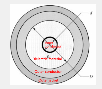
Figure 1.1 Structure of an RF Coaxial Cable

“Characteristic impedance” is one of the most commonly referenced specifications for RF coaxial cables. Maximum power transfer and minimum signal reflection depend on the impedance match between the cable and other components in the system. If the impedance is perfectly matched, the only loss in the cable is the attenuation along the transmission line, without any reflection loss.

The characteristic impedance (Z) of a coaxial cable is determined by the ratio of the inner and outer conductor dimensions and the dielectric constant of the filling material. Due to the “skin effect” of RF energy transmission, the critical dimensions for impedance are the outer diameter of the inner conductor and the inner diameter of the outer conductor.

The characteristic impedance can be expressed by the following formulas:

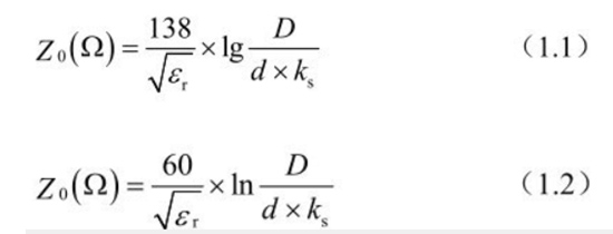
Where:

• Z0 Characteristic impedance in ohms (Ω)
• εr Relative dielectric constant of the dielectric material
• D Inner diameter of the outer conductor (mm)
• d outer diameter of the inner conductor (mm)
• ks inner conductor coefficient, dependent on its structure:
• ks​=1 for a solid center conductor,
• ks​=0.939 for a 7-strand conductor,
• ks​=0.97 for a 19-strand conductor.

Take the semi-rigid coaxial cable EZ141-AL-TP/M17 from Huber+Suhner as an example. From the product datasheet, the inner conductor diameter d=0.92 mm, the outer conductor inner diameter D=2.99 mm, and the dielectric material is PTFE (polytetrafluoroethylene), with εr​=2. Since the inner conductor is a single solid wire, ks​=1. Applying Equation (1.1), the calculated characteristic impedance is 49.95 Ω.

Deviation of Characteristic Impedance

Most RF coaxial cables are designed for a characteristic impedance of 50 Ω. However, in the above example, the calculated value of the EZ141-AL-TP/M17 is not exactly 50 Ω. Why is this?

Equations (1.1) and (1.2) indicate that the characteristic impedance of a coaxial cable depends on three parameters: the inner diameter of the outer conductor D, the outer diameter of the inner conductor d, and the dielectric constant εr​. To ensure accurate impedance, these three parameters must be tightly controlled during manufacturing. While the physical dimensions D and d can be precisely controlled, the dielectric constant εr​ of the dielectric material is more difficult to control between production batches.

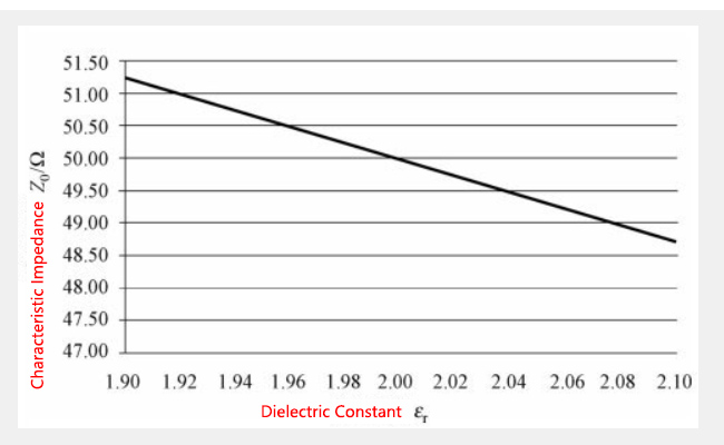
For example, the dielectric constant of PTFE typically ranges from 2.0 to 2.1. Using the same physical dimensions of the EZ141-AL-TP/M17, the calculated characteristic impedance would range from 49.95 Ω to 48.75 Ω. Figure below shows the relationship between the dielectric constant and the characteristic impedance for fixed values of D and d.

Typically, RF coaxial cable datasheets specify the allowable deviation in characteristic impedance (e.g., 50 Ω ± 2%), but only the type of dielectric material is listed, without providing the actual dielectric constant.

Why 50 Ω Characteristic Impedance?

Coaxial cables are available with characteristic impedances of 25 Ω, 50 Ω, 75 Ω, 93 Ω, etc., but 50 Ω is the most widely used standard. Why?

It is commonly believed that a larger conductor cross-section results in lower loss, but this is not entirely true. The loss per unit length in coaxial cables is a function of the ratio D/d, which is directly related to the characteristic impedance.

Calculations show that the minimum loss per unit length does not occur when the inner conductor is at its maximum diameter, but rather when the ratio D/d is approximately 3.6. At this ratio, the characteristic impedance is approximately 77 Ω.

For air-dielectric coaxial cables, breakdown occurs when the maximum electric field strength EE reaches approximately 2.9 × 10⁴ V/cm. Calculations also show that maximum power capacity is achieved when the ratio D/d is approximately 1.65, corresponding to a characteristic impedance of 30 Ω.

To balance minimum loss and maximum power capacity, an optimal impedance value should be selected between 77 Ω and 30 Ω. The arithmetic mean of these two values is 53.5 Ω, while the geometric mean is 48.06 Ω. A 50 Ω impedance is chosen as a compromise between the two. Additionally, 50 Ω RF connectors are easier to design and manufacture.

Most RF cables used in communication systems have a characteristic impedance of 50 Ω, while 75 Ω cables are typically used in broadcast and television applications.

Most test instruments have a 50 Ω impedance. When measuring 75 Ω devices, an impedance transformer (50 Ω to 75 Ω) can be used, but it introduces approximately 5.7 dB of insertion loss.

Capacitance and Inductance

Like characteristic impedance, the per-unit-length capacitance (C) and inductance (L) of a coaxial cable depend on the ratio of the conductor diameters D/d and the dielectric constant εr​.

Voltage Standing Wave Ratio (VSWR) / Return Loss

In RF and microwave systems, maximum power transfer and minimum signal reflection depend on the impedance match between the cable and other system components. Variations in the cable’s impedance cause signal reflections, leading to a loss of incident wave energy.

Reflections are typically expressed using the Voltage Standing Wave Ratio (VSWR), defined as the ratio of incident to reflected voltage.

Equivalent parameters of VSWR include return loss, reflection coefficient, mismatch loss, and matching efficiency.

The VSWR of a coaxial cable assembly depends on the cable itself, the connectors, and the assembly process. A typical VSWR value for a test cable assembly is less than 1.15, which corresponds to a return loss of 23 dB, meaning the transmission (matching) efficiency is 99.5%. For transmission (S21) testing, a VSWR of less than 1.2 is generally sufficient. However, for reflection (S11) testing, a higher VSWR performance is required. Typically, the return loss of the test system should be at least 10 dB higher than that of the device under test (DUT).

In terms of cable types, semi-rigid and semi-flexible cables generally offer excellent VSWR performance. A standard 0.141″ or 0.086″ cable can achieve a VSWR of less than 1.2 across the DC to 18 GHz range without excessive cost, provided that the assembly and soldering techniques are well controlled.

Achieving low VSWR in flexible cables is more challenging, especially under bending conditions. To balance flexibility and RF performance, flexible test cables with excellent RF characteristics often come at a higher cost.

Experienced RF engineers often lightly flex the cable while measuring S11 with a network analyzer to observe whether the VSWR changes, as a means of evaluating the cable assembly’s performance.

Flexible test cable assemblies are typically categorized by frequency ranges such as 3 GHz, 6 GHz, 13 GHz, 18 GHz, 26.5 GHz, 40 GHz, and 50 GHz.

For higher-frequency applications, microwave test cable assemblies are required, which usually involve more advanced design and manufacturing techniques. These cables often use multi-layer shielding and low-density PTFE (LD-PTFE) as the dielectric material, with dielectric constants ranging from 1.38 to 1.73. This results in a phase velocity exceeding 80% of the speed of light in air, closely approximating air as a dielectric medium.

With technological advancements, microwave test cable assemblies are becoming more cost-effective. For example, the BXT TC13 series is a low-cost microwave test cable designed for measurements up to 12.75 GHz. It uses unsplined N-type connectors made of stainless steel and achieves a VSWR of less than 1.2 up to 13 GHz. An additional stainless steel armor jacket extends the cable’s service life.

Shielding

The shielding effectiveness of coaxial cables depends on the structure of the outer conductor. Several common types of shielding are shown in Figure below.

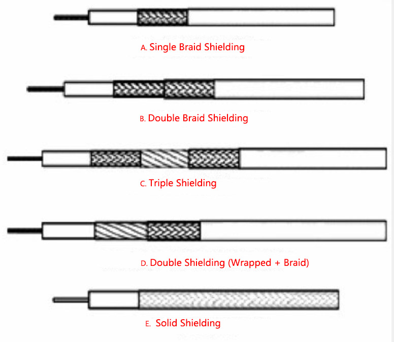
Shielding methods of coaxial cable

• Single Braid Shielding: Coverage ranges from 70% to 95%. Typical products include RG58, RG316 (MIL-C-17), and SV-50-7 (national standard). Shielding effectiveness is approximately -50 dB. Single-layer shielding is suitable for frequencies below 1 GHz. It is not recommended for RF test and measurement applications due to potential electromagnetic leakage.
• Double Braid Shielding: Two layers of braided shielding provide shielding effectiveness from -75 dB to -85 dB. This is the most widely used in general RF testing. Examples include RG316D, RG223, RG142, and RG214.
• Triple Shielding: Two braid layers with an intermediate foil shield, or sometimes a wrapped copper tape as the first layer. Shielding effectiveness ranges from -90 dB to -100 dB. This type is used in EMC and microwave applications, such as Harbour’s LL series.
• Double Shielding (Wrapped + Braid): The inner layer is wrapped silver-plated copper tape, and the outer layer is braided. 100% coverage provides shielding effectiveness of -100 dB. Used in microwave cables such as Micro-Coax’s UTiFLEX series, with operating frequencies up to 40 GHz.
• Solid Shielding: Made from aluminum or copper tubes, offering 100% coverage and shielding effectiveness better than -120 dB at 18 GHz. Examples include Suhner’s EZ141 semi-rigid cable. These cables are formed once and used for internal interconnects where shielding is critical, such as in passive intermodulation (PIM) measurement systems. Corrugated cables are another type of solid shielding, easier to bend, and commonly used in antenna and feeder systems.

Attenuation (Insertion Loss)

Attenuation in coaxial cables indicates the cable’s ability to effectively transmit RF signals and consists of three components: conductor loss, dielectric loss, and radiation loss.

• Conductor Loss is caused by the skin effect and increases with the square root of frequency.
• Dielectric Loss is due to the resistivity of the dielectric material and increases linearly with frequency.
• Radiation Loss results from leakage and is typically negligible except in specialized leaky cables.

Most of the loss is converted into heat. At a given frequency, larger conductor sizes result in lower loss. However, at higher frequencies, dielectric loss becomes more significant. Additionally, increased temperature raises conductor resistance and dielectric loss tangent, increasing overall loss.

Power Handling

Power handling is a key concern in RF cable applications. It is categorized into peak power and average power handling.

• Peak Power Handling is determined by the maximum voltage the cable can withstand.
• Average Power Handling refers to the cable’s ability to dissipate heat generated by conductor and dielectric losses.

Cable cooling is influenced by thermal resistance, which depends on surface area, surface temperature, ambient temperature, thermal conductivity, and airflow.

The maximum operating temperature of the dielectric material determines the cable’s power handling capability, as most heat is generated in the inner conductor. Power handling also depends on altitude:

Pa = Pavg * Ft *Fa

Where:

• Pa​: Effective power capacity
• Pavg​: Rated average power
• Ft​: Temperature factor
• Fa​: Altitude factor

Example: RG393 cable has an average power capacity of 2800 W at 400 MHz, 25 °C, and sea level. At 3048 m altitude, the average power capacity drops to 2520 W (2800*1*0.9 =2520). This consideration is important for high-altitude or aerospace applications.

RF power is often expressed in dBm, which simplifies power calculations.

Propagation Velocity

Propagation velocity, also known as velocity factor (VF), is the ratio of the signal propagation speed in the cable to the speed of light in a vacuum. It is determined by the dielectric constant εr​:

Vp (%) =1 \ √εr *100%
As can be seen from the above formula, the smaller the dielectric constant (εr), the closer the propagation velocity (Vp) is to the speed of light. Therefore, cables with low-density dielectric materials exhibit lower insertion loss.

The phase velocity specification of a cable is of particular importance to RF test engineers. In addition to indicating the cable’s loss characteristics, it enables fault detection in long cables using DTF (Distance to Fault) measurement techniques. Instruments equipped with DTF functionality include Bird Electronic’s SA series antenna and cable analyzers and Wiltron’s Site Master series transmission line and antenna analyzers. These handheld instruments contain built-in signal sources that send a signal through the cable. When the signal encounters a fault (impedance mismatch), part of the signal is reflected back to the instrument. Based on the round-trip transmission time, the instrument calculates the location of the fault. Prior to testing, the dielectric constant of the cable—or equivalently, the signal propagation velocity—must be entered into the instrument to ensure accurate measurement results.

Figure below shows an example of DTF testing on a cellular base station antenna and feeder system. On the horizontal axis, the starting point is the location of the transmitter and cable analyzer. The 0 ft (1 ft = 0.3048 m) position represents the input port of the feeder with a VSWR of 1.05. The jumper-to-main feeder connection at approximately 9 ft has a VSWR of 1.012. The antenna input at 100 ft has a VSWR of 1.06. Two prominent standing wave points appear around 34 ft and 42 ft. Although the VSWR values are not high, these points may indicate potential faults. Possible causes include deformation of the outer conductor due to over-tightened grounding clamps, moisture ingress into the dielectric, or corrosion caused by damaged insulation layers.

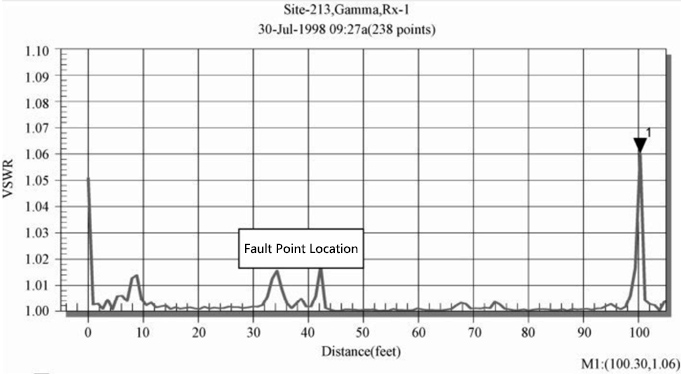
Figure DTF (Distance to Fault) Test of a Cable

Electrical Length

Understanding propagation velocity facilitates comprehension of the concept of electrical length. Electromagnetic waves travel in air at nearly the speed of light, but propagate slower through cable dielectrics. Therefore, the electrical length of a cable is longer than its physical length.

Electrical Length = Physical Length / Vp (%)

In array antenna systems, multiple RF cable assemblies are used to deliver signals from the feed network to the antenna elements. These cables must meet strict electrical length requirements; otherwise, antenna beamforming and directional characteristics may be distorted.

Electrical length can also be expressed in terms of propagation delay, insertion phase, time delay, line length, or dielectric wavelength, in addition to phase velocity.

The phase stability of electrical length is temperature-dependent. Cables with PTFE dielectric exhibit superior phase stability compared to those with polyethylene (PE) dielectric.

Cable Bending Characteristics

For RF test cable assemblies, bending characteristics are crucial to maintaining test accuracy, as bending can cause variations in VSWR, loss, and phase.

Each coaxial cable has a minimum bend radius specification, which is categorized into static and dynamic types. For example, according to MIL-C-17, the RG223/U cable with an outer diameter of 5.4 mm has a minimum static bend radius of 30 mm and a dynamic bend radius of 54 mm. In practical test applications, it is recommended that the minimum bend radius should not be less than 10 times the cable diameter.

In test cable assemblies, the workmanship at the connector-to-cable junction significantly affects the stability of VSWR and insertion loss. From this perspective, the anti-bending design at the connector-to-cable interface is an important criterion for evaluating and selecting RF test cables. Common heat-shrink tubing does not provide effective bend protection. Better solutions include rigid strain reliefs or stainless steel armored jackets with heat-shrink tubing. These methods offer effective protection for the connector-to-cable junction, preventing excessive bending. Testing shows that even after connector wear, the cable base remains intact with this design.

In microwave testing applications, cables are required to maintain minimal phase change under bending—these are known as “phase-stable cables.” In general, cables with foamed dielectrics exhibit better phase stability than those with solid dielectrics. Additionally, cables with stranded inner conductors offer better phase stability than those with solid inner conductors. In some applications, phase stability under bending is a critical performance metric for microwave cables. For example, microwave cables with an outer diameter of approximately 5 mm, when bent to a diameter of 50 mm, typically exhibit phase variations between 2° and 5°.

Passive Intermodulation (PIM) Characteristics of Coaxial Cables

Passive intermodulation (PIM) distortion in cables arises from internal nonlinearities. In an ideal linear system, the output signal is identical to the input signal. However, in nonlinear systems, amplitude distortion occurs. When two or more signals pass through a nonlinear system, intermodulation products are generated. In modern communication systems, third-order intermodulation products (e.g., 2* f1-f2 or 2* f2-f1) are of particular concern, as these unwanted frequency components can fall within receive or transmit bands and cause interference.

Although coaxial cable assemblies are generally considered linear components, perfect linearity does not exist. Nonlinearities typically originate from skin effect, surface oxidation, or poor contact at connector interfaces. The following design guidelines can help minimize PIM:

1. Use semi-rigid or semi-flexible cables instead of flexible cables within equipment.
2. Ensure sufficient plating thickness on conductor surfaces.
3. Use cables with solid inner conductors.
4. Use high-quality connectors with smooth surfaces.
5. Use connectors with thick and uniform plating.
6. Use larger connectors (e.g., DIN 7-16 has better PIM performance than N-type, which in turn outperforms SMA).
7. Ensure good contact between connectors.
8. Use non-magnetic connector materials.

Among commonly used RF coaxial cables, semi-rigid and semi-flexible cables typically exhibit excellent PIM performance, achieving values better than -163 dBc (2*43 dBm). Corrugated cables also offer similar performance, whereas standard braided cables typically exhibit PIM levels below -140 dBc. Manufacturing high-performance low-PIM test cables is challenging, and maintaining their performance over time also depends heavily on proper handling and usage.

1.2 Classification and Selection of Coaxial Cables

RF coaxial cables are categorized into semi-rigid, semi-flexible, flexible (braided), and corrugated types. The appropriate type should be selected based on application requirements. Semi-rigid and semi-flexible cables are commonly used for internal equipment interconnects, while flexible cables are preferred for test and measurement applications. Corrugated cables are typically used in antenna and feeder systems.

Semi-Rigid Cable

As the name implies, semi-rigid cables are not easily bent. Their outer conductors are made of aluminum or copper tubes, resulting in minimal RF leakage (less than -120 dB), making signal crosstalk negligible in systems. These cables also exhibit excellent PIM performance. To bend them into a specific shape, specialized forming machines or manual dies are required. Despite the complex manufacturing process, semi-rigid cables offer excellent performance stability. They typically use solid PTFE as the dielectric, which provides excellent temperature and phase stability, particularly under high-temperature conditions.

Semi-rigid cables are more expensive than semi-flexible cables and are widely used in RF and microwave systems.

Semi-Flexible Cable

In some cases, semi-flexible cables serve as alternatives to semi-rigid cables. They offer performance close to semi-rigid cables and can be manually shaped. However, their mechanical and electrical stability is slightly inferior. Their ease of forming also makes them prone to deformation, especially after prolonged use. (RG402 / RG405 Semi-rigid Coaxial Cable)

Flexible (Braided) Cable

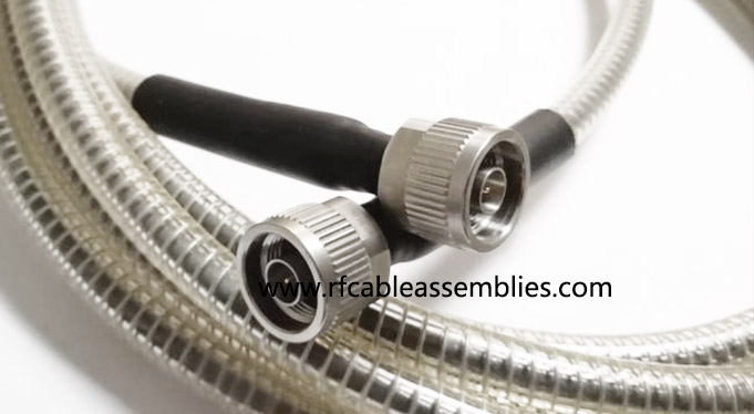
Most “test-grade” cable assemblies use flexible cables (see Figure 1.12). Compared to semi-rigid and semi-flexible cables, flexible cables are more expensive due to the greater number of design considerations. Flexible cables must maintain performance after repeated bending, which is the basic requirement for test cables. Flexibility and good electrical performance are inherently conflicting, which also contributes to their high cost.

When selecting flexible RF cable assemblies, multiple factors must be considered. Some of these factors are contradictory. For example, cables with solid inner conductors have lower insertion loss and better amplitude stability under bending than stranded conductor cables, but exhibit inferior phase stability. Therefore, cable selection should take into account not only frequency range, VSWR, and insertion loss, but also mechanical properties, environmental conditions, and application requirements. Cost is also always a key consideration.

Corrugated Cable

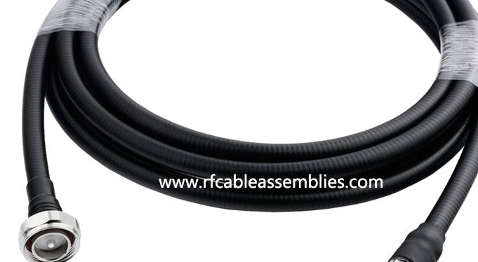
The outer conductor of a corrugated cable is a corrugated copper tube (sometimes aluminum). These cables are designed for low loss and are commonly used in antenna and feeder systems.

The corrugated outer conductor design offers advantages such as ease of bending and transport, as well as excellent tensile strength, making them suitable for vertical suspension applications.

1.3 Execution Standards for Coaxial Cables

The use of coaxial cables is not isolated. In addition to meeting impedance standards, another important constraint is their compatibility with connectors. After decades of development, the mainstream standard for general-purpose RF cables has tended toward the U.S. Military Specification MIL-C-17. Major connector manufacturers also design corresponding connectors based on the RG series cables that conform to the MIL-C-17 standard.

Low-Loss RF Coaxial Cables

In high-power signal transmission applications, reducing cable loss is more cost-effective than increasing transmitter power. Therefore, cable designers continuously optimize parameters to achieve lower loss. The most effective way to reduce loss is to lower the dielectric constant of the filling material. In extreme cases, such as in broadcast transmission systems, air-dielectric cables are used with PTFE support rods to fix the inner conductor, achieving a dielectric constant close to 1.

In mobile communications, physically foamed polyethylene (PE) is commonly used as the dielectric material, with a dielectric constant ranging from 1.29 to 1.64. When εr is reduced, maintaining a 50 Ω characteristic impedance becomes a challenge. As shown in Equation (1.1), reducing εr requires a reduction in ln(D/d). A common approach is to increase the inner conductor diameter (d). However, this can make the cable incompatible with standard connectors, leading to the development of new cable and connector series.

There is no universal standard for low-loss coaxial cables, and market demand typically drives development. Representative products include Times Microwave Systems’ LMR series, Andrew’s LDF series, and RFS’s LCF series.

Microwave Coaxial Cables

For microwave frequencies above 18 GHz, there are no universally accepted standards. This domain is highly fragmented, with each manufacturer following its own internal specifications. Most microwave cables use low-density PTFE dielectrics with εr ranging from 1.38 to 1.73. With similar outer conductor dimensions, microwave cables typically have larger inner conductors than standard RG cables. Rarely do microwave cable manufacturers publicly disclose the exact inner and outer conductor dimensions in their product catalogs.

1.4 Selection of Test Cable Assemblies

Based on the previous discussion, the following principles can be summarized for selecting RF test cable assemblies. (SMA cables , BNC Cables , MMCX Cables )

Adequacy Principle

When selecting test cables, the principle of adequacy should be followed—there is no need to blindly pursue high-performance cables if lower-performance options are sufficient for the application. For example:

• When measuring in-band parameters of cellular mobile communication equipment, a test cable assembly with an upper frequency limit of 3 GHz is sufficient.
• For measuring conducted spurious emissions up to 12.75 GHz, a cable assembly rated to 13 GHz is adequate—there is no need to select one rated to 18 GHz.
• For routine S₁₁ and S₂₂ measurements of passive components, standard RF cables with PE (polyethylene) or solid PTFE (polytetrafluoroethylene) dielectric are sufficient-there is no need to use microwave cables with low-density PTFE (LD-PTFE) dielectric.
• When measuring passive intermodulation (PIM) of ferrite components, RG142 cable is sufficient—there is no need to use specialized low-PIM cables.

Balancing Flexibility and Electrical Performance

Many RF test engineers consider flexibility as one of the key criteria when purchasing test cables. However, this often comes at a higher cost. In general, to maintain both flexibility and electrical performance:

• Solid dielectric materials such as solid PE or solid PTFE are not suitable.
• Instead, cables with low-density PTFE (LD-PTFE) dielectric are used to achieve better flexibility.
• Additional design considerations in the braid layer and jacket are also required to maintain performance, all of which contribute to higher manufacturing costs.

For low-PIM cable assemblies, flexibility becomes even more difficult to maintain.

Cables with solid PE or PTFE dielectric and an outer diameter of less than 5 mm typically offer acceptable flexibility for most applications.

VSWR Specification

VSWR is an important specification for test cables, and users generally prefer lower values. However, due to the inherent randomness in VSWR measurements, manufacturers are often reluctant to guarantee very low VSWR values. To address this:

• It is common practice to specify both a guaranteed value and a typical value.
• For example, a cable may have a guaranteed VSWR of 1.25, while the typical measured value is less than 1.1.
• This approach provides users with sufficient information for cable selection.

Insertion Loss

In most test applications, insertion loss can be calibrated out, so there is generally no need to pursue ultra-low-loss cables unless the application involves high-power transmission. Insertion loss is closely related to cost, and cables with lower loss typically have larger diameters, which conflicts with the requirement for flexibility.

Service Life of Test Cable Assemblies

RF cable assemblies for test are frequently used and must withstand repeated connections and disconnections. Their service life is primarily determined by the number of mating cycles the connectors can endure.

• For example, according to MIL-39012, the rated mating life of an N-type connector is 500 cycles. However, in practical use, the actual life often exceeds this number significantly.
• In one experiment, after 2000 mating cycles, the increase in insertion loss was less than 0.2 dB, and the VSWR remained nearly unchanged.